Sound

Generating sounds

The Sound class provides methods for generating, manipulating, displaying, and analysing sound stimuli. You can generate typical experimental stimuli with this class, including tones, noises, and click trains, and also more specialized stimuli, like equally-masking noises, Schroeder-phase harmonics, iterated ripple noise and synthetic vowels. Slab methods assume sensible defaults where possible. You can call most methods without arguments to get an impression of what they do (f.i. slab.Sound.tone() returns a 1s-long 1kHz tone at 70 dB sampled at 8 kHz) and then customise from there. For instance, let’s make a 500 ms long 500 Hz pure tone signal with a band-limited (one octave below and above the tone) pink noise background with a 10 dB signal-to-noise ratio:

tone = slab.Sound.tone(frequency=500, duration=0.5)
tone.level = 80 # setting the intensity to 80 dB
noise = slab.Sound.pinknoise(duration=0.5)
noise.filter(frequency=(250, 1000), kind='bp') # bandpass .25 to 1 kHz
noise.level = 70 # 10 dB lower than the tone
stimulus = tone + noise # combine the two signals
stimulus = stimulus.ramp() # apply on- and offset ramps to avoid clicks
stimulus.play()

Sound objects have many useful methods for manipulating (like ramp(), filter(), and pulse()) or inspecting them (like waveform(), spectrum(), and spectral_feature()). A complete list is in the Reference documentation section, and the majority is also discussed here. If you use IPython, you can tap the tab key after typing slab.Sound., or the name of any Sound object followed by a full stop, to get an interactive list of the possibilities.

Sounds can also be created by recording them with slab.Sound.record(). For instance recording = slab.Sound.record(duration=1.0, samplerate=44100) will record a 1-second sound at 44100 Hz from the default audio input (usually the microphone). The record method uses SoundCard if installed, or SoX (via a temporary file) otherwise. Both are cross-platform and easy to install. If neither tool is installed, you won’t be able to record sounds.

Specifying durations

Sometimes it is useful to specify the duration of a stimulus in samples rather than seconds. All methods that generate sounds have a duration argument that accepts floating point numbers or integers. Floating point numbers are interpreted as durations in seconds (slab.Sound.tone(duration=1.0) results in a 1 second tone). Integers are interpreted as number of samples (slab.Sound.tone(duration=1000) gives you 1000 samples of a tone).

Setting the sample rate

We did not specify a sample rate for any of the stimuli in the examples above. When the samplerate argument of a sound-generating method is not specified, the default sample rate (8 kHz if not set otherwise) is used. It is possible to set a sample rate separately for each Sound object, but it is usually better to set a suitable default sample rate at the start of your script or Python session using slab.set_default_samplerate(). This rate is kept in the class variable _default_samplerate and is used whenever you call a sound generating method without specifying a rate. This rate depends on the frequency content of your stimuli and should be at least double the highest frequency of interest. For some speech sounds or narrow bad noises you might get away with 8 kHz; for spatial sounds you may need 48 kHz or more.

Specifying levels

Same as for the sample rate, sounds are generated at a default level (70 dB if not set otherwise). The default is kept in the class variable _default_level and you can set set it to a different value using slab.set_default_level(). Level are not specified directly when generating sounds, but rather afterwards by setting the level property:

sig = slab.Sound.pinknoise()
sig.level # return the current level
sig.level = 85 # set a new level

Note that the returned level will not be the actual physical playback level, because that depends on the playback hardware (soundcard, amplifiers, headphones, speakers). Calibrate your system if you need to play stimuli at a known level (see Calibrating the output).

Calibrating the output

Analogous to setting the default level at which sounds are generated with slab.set_default_level(). Each sound’s level can be set individually by changing its level property. Setting the level property of a stimulus changes the root-mean-square of the waveform and relative changes are correct (reducing the level attribute by 10 dB will reduce the sound output by the same amount), but the absolute intensity is only correct if you calibrate your output. The recommended procedure it to set your system volume to maximum, connect the listening hardware (headphone or loudspeaker) and set up a sound level meter. Then call slab.calibrate(). The calibrate() function will play a 1 kHz tone for 5 seconds. Note the recorded intensity on the meter and enter it when requested. The function returns a calibration intensity, i.e. difference between the tone’s level attribute and the recorded level. Pass this value to slab.set_calibration_intensity() to to correct the intensities returned by the level property all sounds. The calibration intensity is saved in the class variable _calibration_intensity. It is applied to all level calculations so that a sound’s level attribute now roughly corresponds to the actual output intensity in dB SPL—‘roughly’ because your output hardware may not have a flat frequency transfer function (some frequencies play louder than others). See Filters for methods to equalize transfer functions.

Experiments sometimes require you to play different stimuli at comparable loudness. Loudness is the perception of sound intensity and it is difficult to calculate. You can use the Sound.aweight() method of a sound to filter it so that frequencies are weighted according to the typical human hearing thresholds. This will increase the correspondence between the rms intensity measure returned by the level attribute and the perceived loudness. However, in most cases, controlling relative intensities is sufficient.

To increase the accuracy of the calibration for your experimental stimuli, pass a sound with a similar spectrum to slab.calibrate(). For instance, if your stimuli are wide band pink noises, then you may want to use a pink noise for calibration. The level of the noise should be high, but not cause clipping.

If you do not have a sound level meter, then you can present sounds in dB HL (hearing level). For that, measure the hearing threshold of the listener at the frequency or frequencies that are presented in your experiment and play your stimuli at a set level above that threshold. You can measure the hearing threshold at one frequency (or for any broadband sound) with the few lines of code (see Audiogram).

Saving and loading sounds

You can save sounds to wav files by calling the object’s Sound.write() method (signal.write('signal.wav')). By default, sounds are normalized to have a maximal amplitude of 1 to avoid clipping when writing the file. You should set signal.level to the intended level when loading a sound from file or disable normalization if you know what you are doing. You can load a wav file by initializing a Sound object with the filename: signal = slab.Sound('signal.wav').

Combining sounds

Several functions allow you to string stimuli together. For instance, in a forward masking experiment [1] we need a masking noise followed by a target sound after a brief silent interval. An example implementation of a complete experiment is discussed in the Psychoacoustics section, but here, we will construct the stimulus:

masker = slab.Sound.tone(frequency=550, duration=0.5) # a 0.5s 550 Hz tone
masker.level = 80 # at 80 dB
masker.ramp() # default 10 ms raised cosine ramps
silence = slab.Sound.silence(duration=0.01) # 10 ms silence
signal = slab.Sound.tone(duration=0.05) # using the default 500 Hz
signal.level = 80 # let's start at the same intensity as the masker
signal.ramp(duration=0.005) # short signal, we'll use 5 ms ramps
stimulus = slab.Sound.sequence(masker, silence, signal)
stimulus.play()

We can make a classic non-interactive demonstration of forward masking by playing these stimuli with decreasing signal level in a loop, once without the masker, and once with the masker. Count for how many steps you can hear the signal tone:

import time # we need the sleep function
for level in range(80, 10, -5): # down from 80 in steps of 5 dB
    signal.level = level
    signal.play()
    time.sleep(0.5)
# now with the masker
for level in range(80, 10, -5): # down from 80 in steps of 5 dB
    signal.level = level
    stimulus = slab.Sound.sequence(masker, silence, signal)
    stimulus.play()
    time.sleep(0.5)

Many listeners can hear all of the steps without the masker, but only the first 6 or 7 steps with the masker. This depends on the intensity at which you play the demo (see Calibrating the output below). The sequence() method is an example of list unpacking—you can provide any number of sounds to be concatenated. If you have a list of sounds, call the method like so: slab.Sound.sequence(*[list_of_sound_objects]) to unpack the list into function arguments.

Another method to put sounds together is crossfade(), which applies a crossfading between two sounds with a specified overlap in seconds. An interesting experimental use is in adaptation designs, in which one longer stimulus is played to adapt neuronal responses to its sound features, and then a new stimulus feature is introduced (but nothing else changes). Responses (measured for instance with EEG) at that point will be mostly due to that feature. A classical example is the pitch onset response, which is evoked when the temporal fine structure of a continuous noise is regularized to produce a pitch percept without altering the sound spectrum (see Krumbholz et al. (2003)). It is easy to generate the main stimulus of that study, a noise transitioning to an iterates ripple noise after two seconds, with 5 ms crossfade overlap, then filtered between 0.8 and 3.2 kHz:

slab.set_default_samplerate(16000) # we need a higher sample rate
slab.set_default_level(80)  # set the level for all sounds to 80 dB
adapter = slab.Sound.whitenoise(duration=2.0)
irn = slab.Sound.irn(frequency=125, n_iter=2, duration=1.0) # pitched sound
stimulus = slab.Sound.crossfade(adapter, irn, overlap=0.005) # crossfade
stimulus.filter(frequency=[800, 3200], kind='bp') # filter
stimulus.ramp(duration=0.005) # 5 ms on- and offset ramps
stimulus.spectrogram() # note that there is no change at the transition
stimulus.play() # but you can hear the onset of the regularity (pitch)

Plotting and analysis

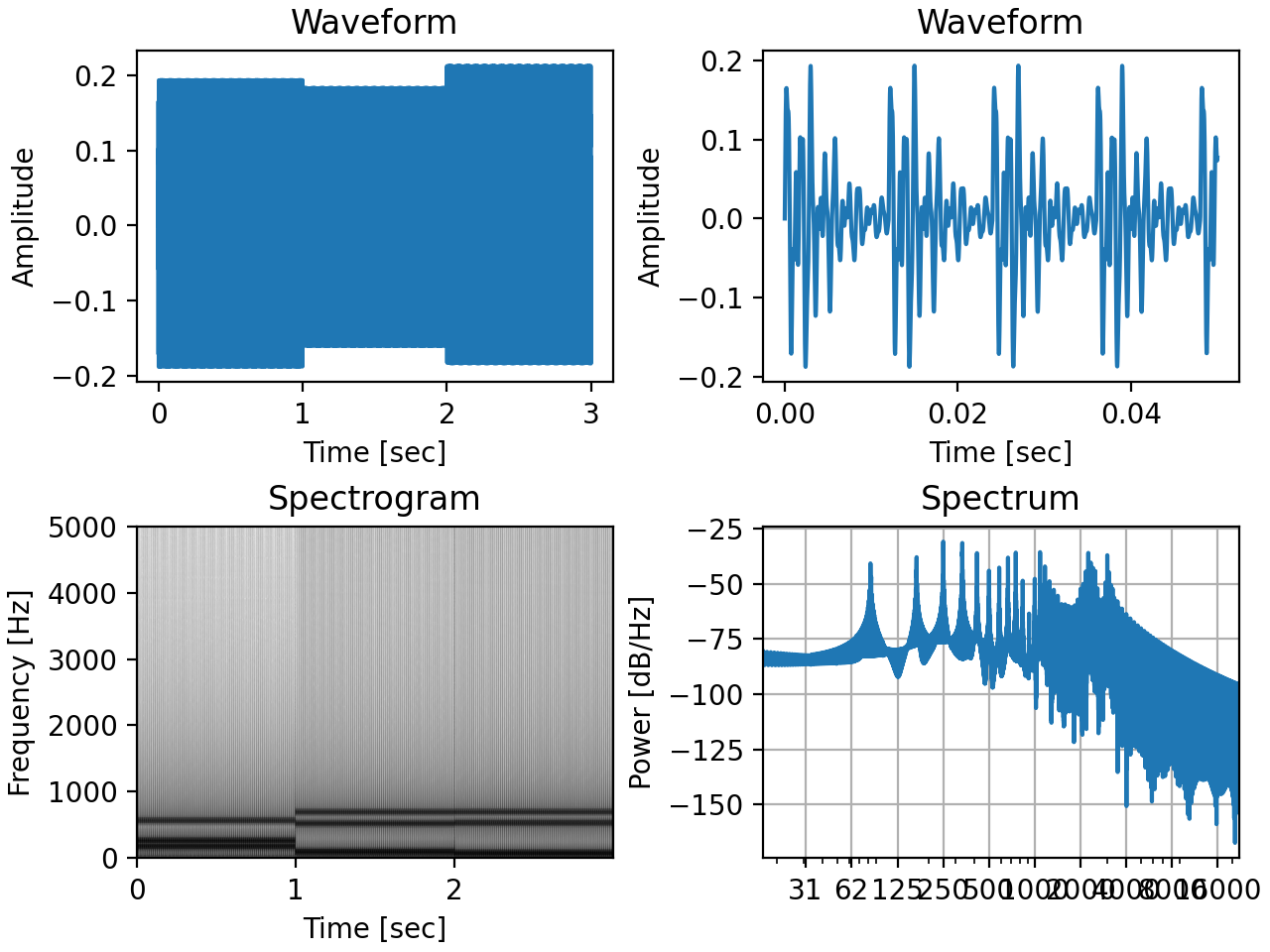
You can inspect sounds by plotting the waveform(), spectrum(), or spectrogram():

from matplotlib import pyplot as plt
a = slab.Sound.vowel(vowel='a')
e = slab.Sound.vowel(vowel='e')
i = slab.Sound.vowel(vowel='i')
signal = slab.Sound.sequence(a,e,i)
import matplotlib.pyplot as plt # preparing a 2-by-2 figure
_, [[ax1, ax2], [ax3, ax4]] = plt.subplots(
                nrows=2, ncols=2, constrained_layout=True)
signal.waveform(axis=ax1, show=False)
signal.waveform(end=0.05, axis=ax2, show=False) # first 50ms
signal.spectrogram(upper_frequency=5000, axis=ax3, show=False)
signal.spectrum(axis=ax4)

(Source code, png, hires.png, pdf)

Instead of plotting, spectrum() and spectrogram() will return the time frequency bins and spectral power values for further analysis if you set the show argument to False. All plotting functions can draw into an existing matplotlib.pyplot axis supplied with the axis argument.

You can also extract common features from sounds, such as the crest_factor() (a measure of how ‘peaky’ the waveform is), or the average onset_slope() (a measure of how fast the on-ramps in the sound are—important for sound localization). Features of the spectral content are bundled in the spectral_feature() method. It can compute spectral centroid, flux, flatness, and rolloff, either for an entire sound (suitable for stationary sounds), or for successive time windows (frames, suitable for time-varying sounds). * The centroid is a measure of the center of mass of a spectrum (i.e. the ‘center’ frequency). * The flux measures how quickly the power spectrum is changing by comparing the power spectrum for one frame against the power spectrum from the previous frame; flatness measures how tone-like a sound is, as opposed to being noise-like, and is calculated by dividing the geometric mean of the power spectrum by the arithmetic mean (see Dubnov (2004)). * The rolloff measures the frequency at which the spectrum rolls off, typically used to find a suitable low-cutoff frequency that retains most of the sound power. These particular features are integrated in slab because we find them useful in our daily work. Many more features are available in packages specialised on audio processing, for instance librosa. librosa interfaces easily with slab, you can just hand the sample data and the sample rate of an slab object separately to most of its methods:

import librosa
sig = slab.Sound('music.wav') # load wav file into slab.Sound object
librosa.beat.beat_track(y=sig.data, sr=sig.samplerate)

When working with environmental sounds or other recorded stimuli, one often needs to compute relevant features for collections of recordings in different experimental conditions. The slab module contains a function slab.apply_to_path(), which applies a function to all sound files in a given folder and returns a dictionary of file names and computed features. In fact, you can also use that function to modify (for instance ramp and filter) all files in a folder.

For other time-frequency processing, the frames() provides an easy way to step through the signal in short windowed frames and compute some values from it. For instance, you could detect on- and offsets in the signal by computing the crest factor in each frame:

from matplotlib import pyplot as plt
signal.pulse() # apply a 4 Hz pulse to the 3 vowels from above
signal.waveform() # note the pulses
crest = [] # the short-term crest factor will show on- and offsets
frames = signal.frames(duration=64)
for f in frames:
    crest.append(f.crest_factor())
times = signal.frametimes(duration=64) # frame center times
import matplotlib.pyplot as plt
plt.plot(times, crest) # peaks in the crest factor mark intensity ramps

Binaural sounds

For experiments in spatial hearing, or any other situation that requires differential manipulation of the left and right channel of a sound, you can use the Binaural class. It inherits all methods from Sound and provides additional methods for generating and manipulating binaural sounds, including advanced interaural time and intensity manipulation.

Generating binaural sounds

Binaural sounds support all sound generating functions with a n_hannels attribute of the Sound class, but automatically set n_channels to 2. Noises support an additional kind argument, which can be set to ‘diotic’ (identical noise in both channels) or ‘dichotic’ (uncorrelated noise). Other methods just return 2-channel versions of the stimuli. You can recast any Sound object as Binaural sound, which duplicates the first channel if n_channels is 1 or greater than 2:

monaural = slab.Sound.tone()
monaural.n_channels
out: 1
binaural = slab.Binaural(monaural)
binaural.n_channels
out: 2
binaural.left # access to the left channel
binaural.right # access to the right channel

Loading a wav file with slab.Binaural('file.wav') returns a Binaural sound object with two channels (even if the wav file contains only one channel).

Manipulating ITD and ILD

The easiest manipulation of a binaural parameter may be to change the interaural level difference (ILD). This can be achieved by setting the level attributes of both channels:

noise = slab.Binaural.pinknoise()
noise.left.level = 75
noise.right.level = 85
noise.level
out: array([75., 85.])

The ild() makes this easier and keeps the overall level constant: noise.ild(10) amplifies the right channel by 5 dB and attenuates the left channel by the same amount to achieve a 10dB level difference. Positive dB values move the virtual sound source to the right and negative values move the source to the left. The pink noise in the example is a broadband signal, and the ILD is frequency dependent and should not be the same for all frequencies. A frequency-dependent level difference can be computed and applied with interaural_level_spectrum(). The level spectrum is computed from a head-related transfer function (HRTF) and can be customised for individual listeners. See HRTFs for how to handle these functions. The default level spectrum is computed form the HRTF of the KEMAR binaural recording mannequin (as measured by Gardener and Martin (1994) at the MIT Media Lab). The level spectrum takes a while to compute and it may be useful to save it. It is a Python dict containing the level differences in a numpy array along with a frequency vector, an azimuth vector, and the sample rate. You can save it for instance with pickle:

import pickle
ils = slab.Binaural.make_interaural_level_spectrum()
pickle.dump(ils, open('ils.pickle', 'wb')) # save using pickle
ils = pickle.load(open('ils.pickle', 'rb')) # load pickle

If the limitations of pickle worry you, you can use numpy.save with a small caveat when loading: numpy.save wraps the dict in an object and we need to remove that after loading with the somewhat strange index [()]:

import numpy
numpy.save('ils.npy', ils) # save using numpy
ils = numpy.load('ils.npy, allow_pickle=True)[()] # load and get the original dict from the wrapping object

If you are unsure which ILD value is appropriate, azimuth_to_ild() can compute ILDs corresponding to an azimuth angle, for instance 45 degrees, and a frequency:

slab.Binaural.azimuth_to_ild(45)
# -9.12  # correct ILD in dB
noise.ild(-9.12)  # apply the ILD

A dynamic ILD, which evokes the perception of a moving sound source, can be applied with ild_ramp(). The ramp is linear from and to a given ILD.

Similar functions exist to manipulate interaural time differences (ITD): itd(), azimuth_to_ild() (using a given head radius), and itd_ramp(). To present a signal from a given azimuth using both cues, use the at_azimuth(), which calculates the correct ILD and ITD for you and applies it.

ITD and ILD manipulation leads to the percept of lateralization, that is, a source somewhere between the ears inside the head. Additional spectral shaping is necessary to generate an externalized percept (outside the head). This shaping can be achieved with the externalize(), which applies a low-resolution HRTF filter (KEMAR by default). Using both ramp functions and externalization, it is easy to generate a convincing sound source movement with pulsed pink noise:

noise = slab.Binaural.pinknoise(samplerate=44100)
from_ild = slab.Binaural.azimuth_to_ild(-90)
from_itd = slab.Binaural.azimuth_to_itd(-90)
to_ild = slab.Binaural.azimuth_to_ild(90)
to_itd = slab.Binaural.azimuth_to_itd(90)
noise_moving = noise.ild_ramp(from_ild, to_ild)
noise_moving = noise_moving.itd_ramp(from_itd, to_itd)
noise_moving.externalize() # apply filter in place
noise_moving.play() # best through headphones

Signals

Sounds inherit from the Signal class, which provides a generic signal object with properties duration, number of samples, sample times, number of channels. The actual samples are kept as numpy array in the data property and can be accessed, if necessary as for instance signal.data. Signals support slicing, arithmetic operations, and conversion between sample points and time points directly, without having to access the data property. The methods resample(), envelope(), and delay() are also implemented in Signal and passed to the child classes Sound, Binaural, and Filter. You do not normally need to use the Signal class directly.

sig = slab.Sound.pinknoise(n_channels=3)
sig.duration
out: 1.0
sig.n_samples
out: 8000
sig.data.shape # accessing the sample array
out: (8000, 3) # which has shape (n_samples x n_channels)
sig2 = sig.resample(samplerate=4000) # resample to 4 kHz
env = sig2.envelope() # returns a new signal containing the lowpass Hilbert envelopes of both channels
sig.delay(duration=0.0006, channel=0) # delay the first channel by 0.6 ms

Footnotes

[1]

Forward masking occurs when a signal cannot be heard due to a preceding masking sound. Typically, three intervals are presented to the listener, two contain only the masker and one contains the masker followed by the signal. The listener has to identify the interval with the signal. The level of the masker is fixed and the signal level is varied adaptively to obtain the masked threshold.