HRTFs
A head-related transfer function (HRTF) describes the impact of the listeners ears, head and torso on incoming sound
for every position in space. Knowing the listeners HRTF, you can simulate a sound source at any position by filtering
it with the transfer function corresponding to that position. The HRTF class provides methods for
manipulating, plotting, and applying head-related transfer functions.
Reading HRTF data
Typically the HRTF class is instantiated by loading a file. The canonical format for HRTF-data is called
sofa (Spatially Oriented Format for Acoustics). To read sofa files, you need to install the h5netcdf module:
pip install h5netcdf. The slab includes a set of standard HRTF recordings from KEMAR (a mannequin for acoustic
recordings) in the folder indicated by the data_path() function. For convenience, you can load this dataset
by calling slab.HRTF.kemar(). Print the resulting object to obtain information about the structure of the
HRTF data
hrtf = slab.HRTF.kemar()
print(hrtf)
# <class 'hrtf.HRTF'> sources 710, elevations 14, samples 710, samplerate 44100.0
Libraries of many other recordings can be found on the website of the sofa file format.
You can read any sofa file downloaded from these repositories by calling the HRTF class with the name of
the sofa file as an argument.
Note
The class is at the moment geared towards plotting and analysis of HRTF files in the sofa format, because we needed that functionality for grant applications. The functionality will grow as we start to record and manipulate HRTFs more often.
Note
When we started to writing this code, there was no python module for reading and writing sofa files. Now that pysofaconventions is available, we will at some point switch internally to using that module as backend for reading sofa files, instead of our own limited implementation.
Plotting sources
The HRTF is a set of many transfer functions, each belonging to a certain sound source position (for example,
there are 710 sources in the KEMAR recordings). You can plot the source positions in 3D with the plot_sources()
to get an impression of the density of the recordings. The red dot indicates the position of the listener and the red
arrow indicates the lister’s gaze direction. Optionally, you can supply a list of source indices which will be
highlighted in red. This can be useful when you are selecting source locations for an experiment and want to confirm
that you chose correctly. In the example below, we select sources using the methods elevation_sources(), which
selects sources along a horizontal sphere slice at a given elevation and cone_sources(), which selects sources
along a vertical slice through the source sphere in front of the listener a given angular distance away from the
midline:
# cone_sources and elevation_sources return lists of indices which are concatenated by adding:
hrtf = slab.HRTF.kemar()
sourceidx = hrtf.cone_sources(0) + hrtf.elevation_sources(0)
hrtf.plot_sources(sourceidx) # plot the sources in 3D, highlighting the selected sources
Try a few angles for the elevation_sources() and cone_sources() methods to understand how selecting
the sources works!
Plotting transfer functions
As mentioned before, a HRTF is collection of transfer functions. Each single transfer function is an instance of the
slab.Filter with two channels - one for each ear. The transfer functions are located in the data
list and the coordinates of the corresponding sources can be found in the sources.cartesian list of the hrtf
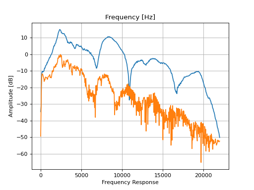
object. In the example below, we select a source, print it’s coordinates and plot the corresponding transfer function.
from matplotlib import pyplot as plt
hrtf = slab.HRTF.kemar()
filt = hrtf.data[10] # choose a filter
source = hrtf.sources.vertical_polar[10]
print(f'azimuth: {round(source[0])}, elevation: {source[1]}')
filt.tf()
(Source code, png, hires.png, pdf)
The HRTF class also has a plot_tf() method to plot transfer functions as either waterfall
(as is Wightman and Kistler, 1989), image plot (as in Hofman 1998). The function takes a list of source indices as an
argument which will be included in the plot. The function below shows how to generate a waterfall and image plot
for the sources along the central cone. Before plotting, we apply a diffuse field equalization to remove non-spatial
components of the HRTF, which makes the features of the HRTF that change with direction easier to see:
hrtf = slab.HRTF.kemar()
fig, ax = plt.subplots(2)
dtf = hrtf.diffuse_field_equalization()
sourceidx = hrtf.cone_sources(0)
ax[0].set_title("waterfall plot")
ax[1].set_title("image plot")
hrtf.plot_tf(sourceidx, ear='left', axis=ax[0], show=False, kind="waterfall")
hrtf.plot_tf(sourceidx, ear='left', axis=ax[1], show=False, kind="image")
plt.tight_layout()
plt.show()
(Source code, png, hires.png, pdf)
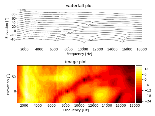
As you can see the HRTF changes systematically with the elevation of the sound source, especially for frequencies above
6 kHz. Individual HRTFs vary in the amount of spectral change across elevations, mostly due to differences in the
shape of the ears. You can compute a measure of the HRTFs spectral dissimilarity the vertical axis, called vertical
spatial information (VSI, Trapeau and Schönwiesner, 2016).
The VSI relates to behavioral localization accuracy in the vertical dimension: listeners with acoustically more
informative spectral cues tend to localize sounds more accurately in the vertical axis. Identical filters give a VSI
of zero, highly dissimilar filters give a VSI closer to one. The hrtf has to be diffuse-field equalized for this
measure to be sensible, and the vsi() method will apply the equalization. The KEMAR mannequin have a VSI
of about 0.73:
hrtf.vsi()
# .73328
The vsi() method accepts arbitrary lists of source indices for the dissimilarity computation.
We can for instance check how the VSI changes when sources further off the midline are used. There are some reports
in the literature that listeners can perceive the elevation of a sound source better if it is a few degrees to the
side. We can check whether this is due to more dissimilar filters at different angles (we’ll reuse the dtf from above
to avoid recalculation of the diffuse-field equalization in each iteration):
for cone in range(0,51,10):
    sources = dtf.cone_sources(cone)
    vsi = dtf.vsi(sources=sources, equalize=False)
    print(f'{cone}˚: {vsi:.2f}')
    # 0˚: 0.73
    # 10˚: 0.63
    # 20˚: 0.69
    # 30˚: 0.74
    # 40˚: 0.76
    # 50˚: 0.73
The effect seems to be weak for KEMAR, (VSI falls off for directions slightly off the midline and then increases again at around 30-40˚).
Applying an HRTF to a monaural sound
The HRTF describes the directional filtering of incoming sounds by the listeners ears, head and torso. Since this is the
basis for localizing sounds in three dimensions, we can apply the HRTF to a sound to evoke the impression of it coming
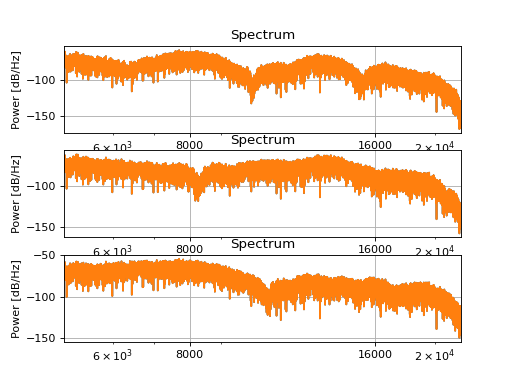
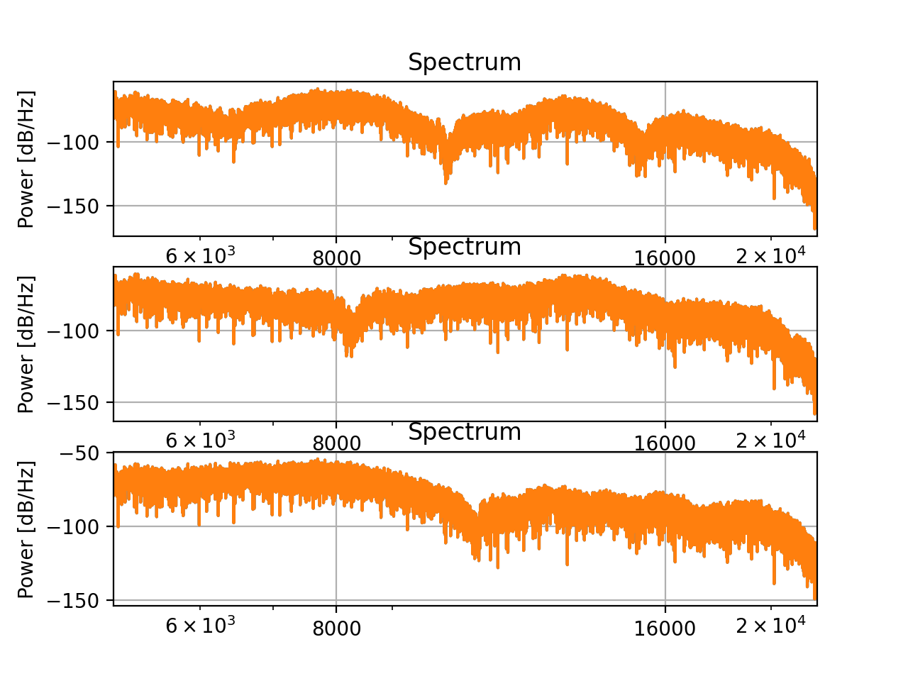
from a certain direction in space when listening through headphones. The HRTF.apply() method returns an instance of
the slab.Binaural. It uses apply() with fir=’IR’, which conserves ITDs. In the example below we
apply the transfer functions corresponding to three sound sources at different elevations along the vertical midline to white noise.
hrtf = slab.HRTF.kemar()
sound = slab.Sound.pinknoise(samplerate=hrtf.samplerate)  # the sound to be spatialized
fig, ax = plt.subplots(3)
sourceidx = [0, 260, 536]  # sources at elevations -40, 0 and 40
spatial_sounds = []
for i, index in enumerate(sourceidx):
    spatial_sounds.append(hrtf.apply(index, sound))
    spatial_sounds[i].spectrum(axis=ax[i], low_cutoff=5000, show=False)
plt.show()
(Source code, png, hires.png, pdf)

You can use the play() method of the sounds to listen to them - see if you can identify the virtual sound
source position. Your ability to do so depends on how similar your own HRTF is to that of the the KEMAR artificial head.
Your auditory system can get used to new HRTFs, so if you listen to the KEMAR recordings long enough they will eventually
produce virtual sound sources at the correct locations.
Binaural filters from the KEMAR HRTF will impose the correct spectral profile, but no ITD. After applying an HRTF filter
corresponding to an off-center direction, you should also apply an ITD corresponding to the direction using the
Binaural.azimuth_to_itd() and Binaural.itd() methods.
Finally, the HRTF filters are recorded only at certain locations (710, in case of KEMAR - plot the source locations to
inspect them). You can interpolate a filter for any location covered by these sources with the HRTF.interpolate()
method. It triangulates the source locations and finds three sources that form a triangle around the requested location
and interpolates a filter with a (barycentric) weighted average in the spectral domain. The resulting slab.Filter
object may not have the same overall gain, so remember to set the level of your stimulus after having applied the interpolated HRTF.
Room simulations
The Room class provides methods to simulate directional echos and reverberation in rectangular rooms. It computes lists of reflections, estimates reverberations times, and generates reverberation tail filters and room impulse responses. The main aim is to provide an easy way to add and manipulate reverb to sounds.
Adding reverb to a sound
The quickest way to add some reverb to a sound, using default values where possible, takes just three lines of code:
room = slab.Room()  # generating an echo list for the default room
hrir = room.hrir()  # compute the room impulse response
echos = hrir.apply(sound)  # assuming 'sound' is an slab.Sound object
Initializing a Room object sets the room dimensions and listener coordinates (both in cartesian coordinates), and the sound source location with respect to the listener (in polar coordinates). The default values generate a room of 4 by 5 by 3 m with the listener in the center and a source straight ahead a 1.4 m distance. A list of echo directions in polar coordinates (azimuth, elevation, distance) with respect to the listener is automatically computed using the image source model method, along with corresponding lists of the number of wall and floor reflections for each echo. The genereation of these lists can be controlled by two additional parameters, order (number of times the source is reflected along each wall, default is 2) and max_echos (the length of the returned list, default 50).
In addition, the absorption parameter of the walls can be set to affect the duration of the reverberation tail.
A moving source
Use the set_source() method to change the sound source direction and automatically recompute the echo list (this is done by calling the _simulated_echo_locations() method). Here is an example that moves a source in a circle with 0.5 m radius counter-clockwise around the listener. The sound is a short synthetic vowel:
sig = slab.Binaural.vowel(duration=0.3)
for d in range(0,360,36):
  room.set_source([d, 20, .5])  # change azi, elevation is 20 deg above the head
  hrir = room.hrir(trim=5000)
  rev = hrir.apply(sig)
  rev.level = 70
  rev.play()
(Listen to this example with headphones.) The generated room impulse responses always have excessively long tails. Plot the response like so:
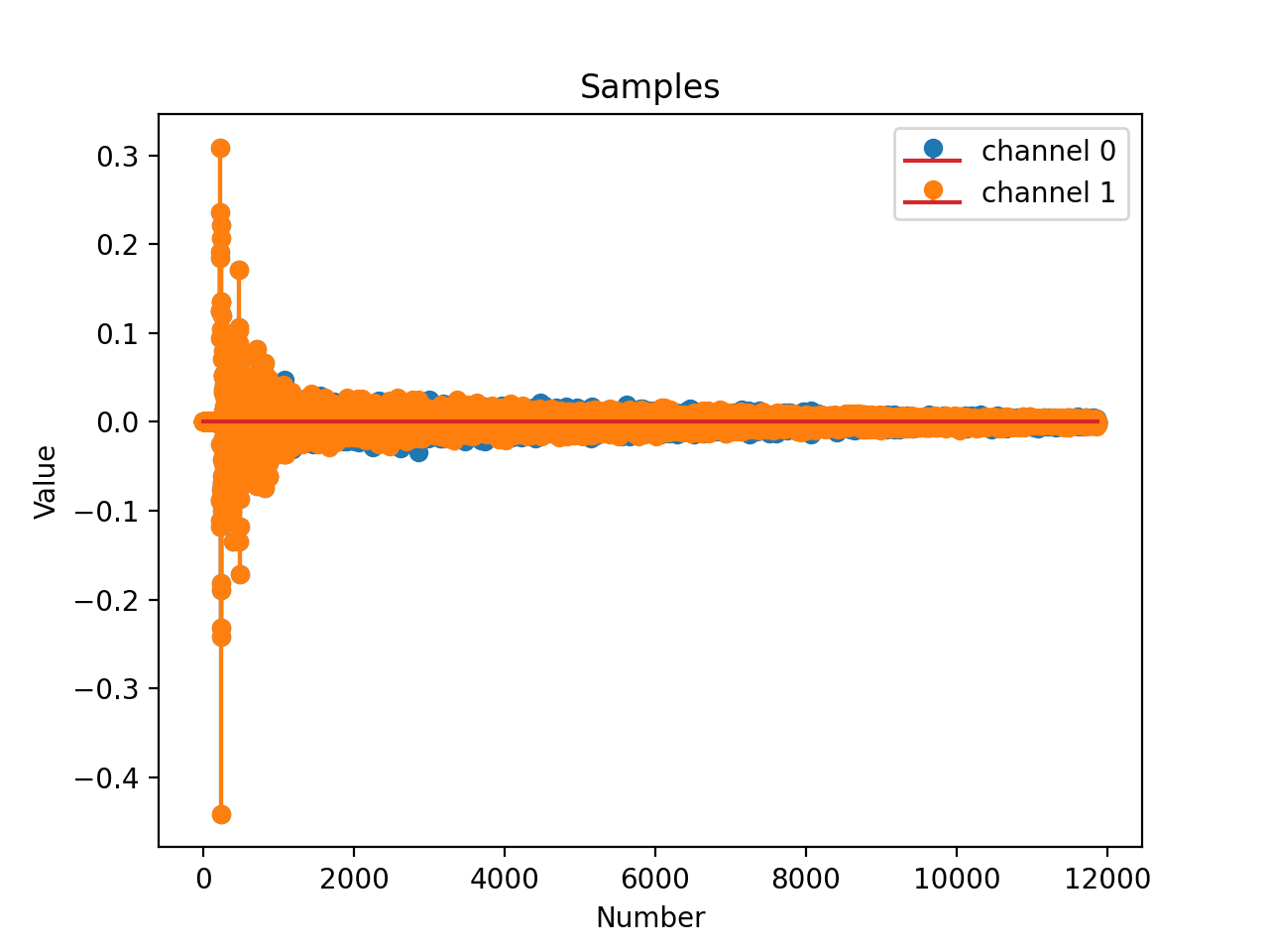
room = slab.Room()
hrir = room.hrir()
hrir.plot_samples()
(Source code, png, hires.png, pdf)
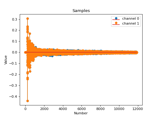
Then determine a suitable cutoff, at which the filter taps are near zero, for instance 20000 samples in this case. You can cut off the filter with the trim argument, which takes an integer and cuts to that number of samples, or a float between 0 and 1 and cuts to that fraction (the default is 0.5, i.e. cut off the second half of the impulse response).
The hrir() method computes the room impulse response by iterating through the echo list and adding the HRTF filter corresponding to each echo direction, delayed and attenuated by the distance of the echo and convolved with the wall or floor material filters, and then adding a noise reverberation tail. The reverberation tail can be provided as an slab.Filter object or will be automatically generated by the reverb() method using the reverb() method to calculate the T60 reverberation time from the room dimensions and absorption coefficient. You can set the HRTF to use with the hrtf argument. The resulting impulse response will have the same samplerate as the hrtf objects (hrtf.samplerate).