Psychoacoustics

The Psychoacoustics class simplifies psychoacoustic experiments by providing classes and methods for trial sequences and adaptive staircases, results and configuration files, response collection via keyboard and button boxes, and handling of collections of precomputed stimuli. This all-in-one approach makes for clean code and easy data management.

Trial sequences

Experiments are often defined by a sequence of trials of different conditions. This sequence is generated before the experiment according to certain rules. In the most basic case, a set of experimental conditions are repeated a number of times pseudorandom order. Such experiments can be handled by the Trialsequence class. To generate an instance of Trialsequence you define a list of conditions and specify how often each of them is repeated (n_reps). You can also specify the kind of list you want to generate: “non_repeating” means that the same condition will not appear twice in a row, “random_permutation” means that the order is completely randomised. For example, generate pure tones with different frequencies and play them in non-repeating, randomised order.:

freqs = [495, 498, 501, 504]  # frequencies of the tones
seq = slab.Trialsequence(conditions=freqs, n_reps=10)  # 10 repetitions per condition
# now we draw elements from the list, generate a tone and play it until we reach the end:
for freq in seq:
  stimulus = slab.Sound.tone(frequency=freq)
  stimulus.play()

Usually, we do not only want to play sounds to the participants in our experiment. Instead, we want them to perform some kind of task and give a response. In the example above we could, for instance, ask after every tone if that tone was higher or lower in frequency than the previous one. The response is captured with the key() context manager which can record single button presses (using either the curses module or the key_press_event() of the stairs plot, see _responses). In our example, we instruct the subject to press “y” (yes) if the played tone was higher then the previous and “n” (no) if it was lower (a 1-back task). After each trial we check if the response was correct and store that information as 1 (correct) or 0 (wrong) in the trial sequence.:

for freq in seq:
  stimulus = slab.Sound.tone(frequency=freq)
  stimulus.play()
  if seq.this_n > 0:  # don't get response for first trial
    previous = seq.get_future_trial(-1)
    with slab.key() as key:  # wait for a key press
      response = key.getch()
    # check if the response was correct, if so store a 1, else store 0
    if (freq > previous and response == ord('y')) or (freq<previous and response == ord('n')):
      seq.add_response(1)
    else:
      seq.add_response(0)
seq.save_json("sequence.json")  # save the trial sequence and response

There are two ways for a response to be correct in this experiment. Either the frequency of the stimulus was higher than the last one and the ‘y’ key was pressed, or it was lower and the ‘n’ key was pressed. (ord() is used to get the key codes of the ‘y’ and ‘n’ keys (112 and 110, respectively). All other options, including missed responses, are counted as wrong answers. Since we encoded correct responses as 1 and wrong responses as 0, we could just sum over the list of responses and divide by the length of the list to get the fraction of trials that was answered correctly.

Kinds of trial sequences

Trial sequences are useful for non-adaptive testing (the current stimulus does not depend on the listeners previous responses) and other situations where you need a controlled sequence of stimulus values. The Trialsequence class constructs several controlled sequences (random permutation, non-repeating, infinite, oddball), computes transition probabilities and condition frequencies, and can keep track of responses:

# sequence of 5 conditions, repeated twice, without direct repetitions:
seq = slab.Trialsequence(conditions=5, n_reps=2)

# infinite sequence of color names:
seq = slab.Trialsequence(conditions=['red', 'green', 'blue'], kind='infinite')

# stimulus sequence for an oddball design:
seq = slab.Trialsequence(conditions=1, deviant_freq=0.12, n_reps=60)

The list of trials is contained in the trials of the Trialsequence object, but you don’t normally need to access this list directly. A Trialsequence object can be used like a Staircase object in a listening experiment and will return the current stimulus value when used in a loop. Below is the detection threshold task from the Staircase, rewritten using Fechner’s method of constant stimuli with a Trialsequence:

stimulus = slab.Sound.tone(duration=0.5)
levels = list(range(0, 50, 10)) # the sound levels to test
trials = slab.Trialsequence(conditions=levels, n_reps=10) # each repeated 10 times
for level in trials:
    stimulus.level = level
    stimulus.play()
    with slab.key() as key:
        response = key.getch()
    trials.add_response(response)
trials.response_summary()

Because there is no simple threshold, the Trialsequence class provides a response_summary(), which tabulates responses by condition index in a nested list.

The infinite kind of Trialsequence is perhaps less suitable for controlling the stimulus parameter of interest, but it is very useful for varying other stimulus attributes in a controlled fashion from trial to trial (think of ‘roving’ paradigms). Unlike when selecting a random value in each trial, the infinite Trialsequence guarantees locally equal value frequencies, avoids direct repetition, and keeps a record in case you want to include the sequence as nuisance covariate in the analysis later on. Here is a real-world example from an experiment with pseudo-words, in which several words without direct repetition were needed in each trial. word_list contained the words as strings, later used to load the correct stimulus file:

word_seq = slab.Trialsequence(conditions=word_list, kind='infinite')
word = next(word_seq) # draw a word from the list

This is one of the very few cases where it makes sense to get the next trial by calling Python’s next() function, because this is not the main trial sequence. The main trial sequence (the one determining the values of your main experimental parameter) should normally be used in a for loop as in the previous example.

Controlling transitions

While randomized sequences do the job most of the time, in some cases it is necessary to control the transitions between the individual conditions more tightly. For instance, you may want to ensure nearly equal transitions, or avoid certain combinations of subsequent conditions entirely. The transitions() method counts, for each condition, how often every other condition follows this one. You can divide the count by the number of repetitions in the sequence to get the transitional probabilities:

trials = slab.Trialsequence(conditions=4, n_reps=10)
trials.transitions()
out:
array([[0., 2., 6., 2.],
       [3., 0., 0., 7.],
       [2., 6., 0., 1.],
       [4., 2., 4., 0.]])
trials.transitions() / 10  # divide by n_reps to get the probability
out:
array([[0. , 0.2, 0.6, 0.2],
       [0.3, 0. , 0. , 0.7],
       [0.2, 0.6, 0. , 0.1],
       [0.4, 0.2, 0.4, 0. ]])

The diagonal of this array contains only zeroes, because a condition cannot follow itself in the default non_repeating trial sequence. The other entries are uneven; for instance, condition 1 is followed by condition 3 seven times, but never by condition 2. If you want near-equal transitions, then you could generate sequences in a loop until a set condition is fulfilled, for instance, no transition > 4:

import numpy
trans = 5
while numpy.any(trans>4):
    trials = slab.Trialsequence(conditions=4, n_reps=10)
    trans = trials.transitions()
print(trans)
out:
array([[0., 3., 3., 3.],
       [4., 0., 3., 3.],
       [3., 4., 0., 3.],
       [3., 3., 4., 0.]])

If your condition is more complicated, you can perform several tests in the loop body and set a flag that determines when all have been satisfied and the loop should be end. But be careful, setting these constraints too tightly may result in an infinite loop.

Alternative Choices

Often, an experimental paradigm requires more complex responses than yes or no. A common option is the classical “forced choice” paradigm, in which the subject has to pick a response from a defined set of responses. Since this is a common paradigm, the Trialsequence and Staircase class have a method for it called present_afc_trial() (afc stands for alternative forced choice). With this function we can make our frequency discrimination task from the example above a bit more elaborate. We define the frequencies of our target tones and add two distractor tones with a frequency of 500 Hz. In each trial, all three tones (target + 2 x distractor) are played in random order. The participant answers the question: “which tone was different from the others?” and responds by pressing the key “1”, “2” or “3”. All of this can be done in only 6 lines of code:

distractor = slab.Sound.tone(duration=0.5, frequency=500)
freqs = list(range(495, 505))
trials = slab.Trialsequence(conditions=freqs, n_reps=2)
for freq in trials:
    target = slab.Sound.tone(frequency=freq, duration=0.5)
    trials.present_afc_trial(target, [distractor, distractor], isi=0.2)

Adaptive staircases

In many cases, you do not want to test every condition with the same frequency, but adapt the stimulus presentation to the responses of the participant. For example, when measuring an audiogram, you want to spend most of the testing time around the threshold to make the testing efficient. The Staircase class lets you do that. You pick an initial value for the stimulus parameter (start_val) and a step size (step_sizes). With each trial, the starting value is decreased by one step size until the subject is not able to respond correctly anymore. Then it is increased step wise until the response is correct again, then decreased again and so on. This procedure is repeated until the given number of reversals (n_reversals) is reached. The step size can be a list in which case the current step size moves one index in the list by each reversal until the end of the list is reached. For example, we could use a step size of 4 until we crossed the threshold for the first time, then use a step size of 1 for the rest of the experiment. This ensures that we get to the threshold quickly and, once we are there, measure it precisely. (The simulate_response() method used here is explained under _simulating.)

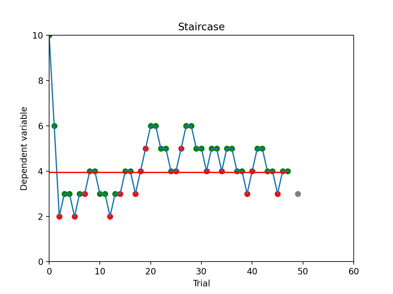
stairs = slab.Staircase(start_val=10, n_reversals=18, step_sizes=[4,1])
for stimulus_value in stairs:
    response = stairs.simulate_response(threshold=3) # simulate subject's response
    stairs.add_response(response) # initiates calculation of next stimulus value
    stairs.plot()

(Source code, png, hires.png, pdf)

Calling the plot function in the for loop (after Staircase.add_response()) will update the plot each trial and let you monitor the performance of the participant, including the current stimulus value (grey dot), and correct/incorrect responses (green and red dots). (On some Windows systems, the plot captures the focus and may prevent you from entering responses in the terminal window. In that case, switch the slab.psychoacoustics.input_method to ‘figure’. This will get a button press through the stairs figure’s key_press_event().)

An audiogram is a typical example for a staircase procedure. We can define a list of frequencies and run a staircase for each one. Afterwards we can print out the result using the thresh() method.:

from matplotlib import pyplot as plt
freqs = [125, 250, 500, 1000, 2000, 4000]
threshs = []
for frequency in freqs:
    stimulus = slab.Sound.tone(frequency=frequency, duration=0.5)
    stairs = slab.Staircase(start_val=50, n_reversals=18)
    print(f'Starting staircase with {frequency} Hz:')
    for level in stairs:
        stimulus.level = level
        stairs.present_tone_trial(stimulus)
    threshs.append(stairs.threshold())
    print(f'Threshold at {frequency} Hz: {stairs.threshold()} dB')
plt.plot(freqs, threshs) # would plot the audiogram

present_tone_trial() is a convenience method that presents the trial, acquires a response, and optionally prints trial information. All of this can be done explicitly, as shown in the Trialsequence example.

Staircase Parameters

Setting up a near optimal staircase requires some expertise and pilot data. Practical recommendations can be found in García-Pérez (1998). start_val sets the stimulus value presented in the first trial and the starting point of the staircase. This stimulus should in general be easy to detect/discriminate for all participants. You can limit the range of stimulus values between min_val and max_val (the default is infinity in both directions). step_sizes determines how far to go up or down when changing the stimulus value adaptively. If it is a list of values, then the first element is used until the first reversal, the second until the second reversal, etc. step_type determines what kind of steps are taken: ‘lin’ adds/subtracts the step size from the current stimulus value, ‘db’ and ‘log’ will step by a certain number of decibels or log units. Typically you would start with a large step size to quickly get close to the threshold, and then switch to a smaller step size. Steps going up are multiplied with step_up_factor to allow unequal step sizes and weighted up-down procedures (Kaernbach (1991)). Optimal step sizes are a bit smaller than the spread of the psychometric function for the parameter you are testing. You can set the number of correct responses required to reduce the stimulus value with ndown and the number of incorrect responses required to increase the value with nup. The default is a 1up-2down procedure. You can also add a number of training trials, in which the stimulus value does not change, with n_pretrials.

Simulating responses

For testing and comparing different staircase settings it can be useful to simulate responses. The first staircase example uses simulate_responses() to draw responses from a logistic psychometric function with a given threshold and width (expressed as the stimulus range in which the function increases from 20% to 80% hitrate). For instance, if the current stimulus value is at the threshold, then the function returns a hit with 50% probability. This is useful to simulate and compare different staircase settings and determine to which hit rate they converge. 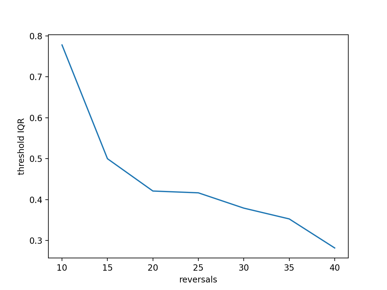For instance, let’s get a feeling for the effect of the length of the measurement (number of reversals required to end the staircase) and the accuracy of the threshold (standard deviation of thresholds across 100 simulated runs). We test from 10 to 40 reversals and run 100 staircases in the inner loop, each time saving the threshold, then computing the interquartile range and plotting it against the number of reversals. Longer measurements should reduce the variability:

from matplotlib import pyplot as plt
stairs_iqr =[]
for reversals in range(10,41,5):
    threshs = []
    for _ in range(100):
        stairs = slab.Staircase(start_val=10, n_reversals=reversals)
        for trial in stairs:
            resp = stairs.simulate_response(3)
            stairs.add_response(resp)
        threshs.append(stairs.threshold())
    threshs.sort()
    stairs_iqr.append(threshs[74] - threshs[24]) # 75th-25th percentile
plt.plot(range(10,41,5), stairs_iqr)
plt.gca().set(xlabel='reversals', ylabel='threshold IQR')

(Source code, png, hires.png, pdf)

Many other useful simulations are possible. You could check whether a 1up-3down procedure procedure would arrive at a similar accuracy in fewer trials, what the best step size for a given psychometric function is, or how much a wider than expected psychometric function increases experimental time. Simulations are a good starting point, but the psychometric function is a very simplistic model for human behaviour. Check the results with pilot data.

Simulation is also useful for finding the hitrate (or point on the psychometric function) that a staircase converges on in cases that are difficult for calculate. For instance, it is not immediately obvious on what threshold a 1up-4down staircase with step_up_factor 1.5 and a 3-alternative forced choice presentation converges on:

import numpy
threshs = []
width = 2
thresh = 3
for _ in range(100):
    stairs = slab.Staircase(start_val=10, n_reversals=30, n_down=4, step_up_factor=1.5)
    for trial in stairs:
        resp = stairs.simulate_response(threshold=thresh, transition_width=width, intervals=3)
        stairs.add_response(resp)
    threshs.append(stairs.threshold())
# now we have 100 thresholds, take mean and convert to equivalent hitrate:
hitrate = 1 / (1 + numpy.exp(4 * (0.5/width)  * (thresh - numpy.mean(threshs))))
print(hitrate)
# 0.83

As you can see, even through the threshold in the response simulation is 3 (that is, the rate of correct responses is > 0.5 above this value; how fast it increases from there depends on the transition_width), the mean threshold returned from the procedure is over 4.5. The last line translates this value in relation to the width of the simulated psychometric function into a hitrate of about 0.83.

Acquiring key presses

When you use a staircase in a listening experiment, you need to record responses from the participant, usually in the form of button presses. The key() context manager can record single button presses from the computer keyboard (or an attached USB number pad), or via the key press event handler of a matplotlib figure, or from a custom USB buttonbox. The input is selected by setting slab.psychoacoustics.input_method to ‘keyboard’, ‘buttonbox’, or ‘figure’. This allow you to test your code on your laptop and switch to button box input at the lab computer by changing a single line of code. Getting a button press from the keyboard will clear your terminal while waiting for the response, and restore it afterwards. The the lab, you may not want to use a keyboard, which can be distracting. A simple response box with the required number of buttons can be constructed easily with an Arduino-compatible micro-controller that can send key codes to the computer via USB. Check for a press of a button attached to a digital input and send a string corresponding to the key code of the desired key followed by the Enter key. If you use the plot() method of the Staircase class to show the progress of the test, you can set the input_method to ‘figure’ to get a keypress via the figure’s key press event handler.

The key() method uses the key code of a button, rather than the string character it produces when pressed. You can find the code of a key by calling Python’s ord() function. For instance, ord(‘y’) returns 121, the code of the ‘y’ key.

The Trialsequence and Staircase classes have two convenience methods to present tones and acquire a response from the listener in one step: present_tone_trial() and present_afc_trial(). Both take a list of key codes that are considered valid responses (:param:`key_codes`). The list defaults to the number keys from 1 to 9. If you use any of these keys in present_tone_trial(), then you just need to specify which of them is counted as a correct response by setting the argument correct_key_idx to the list index that contains the correct key (instead of a single index you can specify a list of indices if you want to count several keys as correct). In present_afc_trial(), the order of the keys in :param:`key_codes` should correspond to the keys that should be pressed to indicate interval 1, 2, etc. In this case, the correct key is different in each trial, depending on the interval that contains the target stimulus.

Here is an example of how to use the key() in a staircase that finds the detection threshold for a 500 Hz tone, after every trial you have to indicate whether you could or could not hear the sound by pressing “y” for yes or any other button for no:

stimulus = slab.Sound.tone(duration=0.5)
stairs = slab.Staircase(start_val=60, step_sizes=[10, 3])
for level in stairs:
    stimulus.level = level
    stimulus.play()
    with slab.key('Press y for yes or n for no.') as key:
        response = key.getch()
    if response == 121:  # 121 is the unicode for the "y" key
        stairs.add_response(True) # initiates calculation of next stimulus value
    else:
        stairs.add_response(False)
stairs.plot()
stairs.threshold()

Note that slab is not optimal for measuring reaction times due to the timing uncertainties in the millisecond range introduced by modern multi-tasking operating systems. If you are serious about reaction times, you should use an external DSP device to ensure accurate timing. Ubiquitous in auditory research are the realtime processors from Tucker-Davies Technologies (our module freefield module works with these devices).

Precomputed sounds

If you present white noise in an experiment, you probably do not want to play the exact same noise in each trial (‘frozen’ noise), but different random instances of noise. The Precomputed class manages a list of pre-generated stimuli, but behave like a single sound. You can pass a list of sounds, a function to generate sounds together with an indication of how many you want, or a generator expression to initialize the Precomputed object. The object has a play() method that plays a random stimulus from the list (but never the stimulus played just before), and remembers all previously played stimuli in the sequence. The Precomputed object can be saved to a zip file and loaded back later on:

# generate 10 instances of pink noise::
stims = slab.Precomputed(lambda: slab.Sound.pinknoise(), n=10)
stims.play() # play a random instance
stims.play() # play another one, guaranteed to be different from the previous one
stims.sequence # the sequence of instances played so far
stims.write('stims.zip') # save the sounds as zip file
stims = slab.Precomputed.read('stims.zip') # reloads the file into a Precomputed object

Results files

In most experiments, the performance of the listener, experimental settings, the presented stimuli, and other information need to be saved to disk during the experiment. The ResultsFile class helps with several typical functions of these files, like generating timestamps, creating the necessary folders, and ensuring that the file is readable if the experiment is interrupted writing to the file after each trial. Information is written incrementally to the file in single lines of JSON (a JSON Lines file).

Set the folder that will hold results files from all participants for the experiment somewhere at the top of your script with the results_folder. Then you can create a file by initializing a class instance with a subject name:

subject_ID = 'MS01'
slab.ResultsFile.results_folder = 'MyResults'
file = slab.ResultsFile(subject='MS')
print(file.name)
file.write(subject_ID)

You can now use the write() method to write any information to the file, to be precise, you can write any object that can be converted to JSON, like strings, lists, or dictionaries. Numpy data types need to be converted to python types. A numpy array can be converted to a list before saving by calling its numpy.ndarray.tolist() method, and numpy ints or floats need to be converted by calling their item() method. You can try out what the JSON representation of an item is by calling:

import json
import numpy
a = 'a string'
b = [1, 2, 3, 4]
c = {'frequency': 500, 'duration': 1.5}
d = numpy.array(b)
for item in [a, b, c]:
    json.dumps(item)
json.dumps(d.tolist())

Trialsequence and Staircase objects can pass their entire current state to the write method, which makes it easy to save all settings and responses from these objects:

trials = slab.Trialsequence(conditions=4, n_reps=10)
file.write(trials, tag='trials')

The write() method writes a dictionary with a single key-value pair, where the key is supplied as tag argument argument (default is a time stamp in the format ‘%Y-%m-%d-%H-%M-%S’), and the value is the json-serialized data you want to save. The information can be read back from the file, either while the experiment is running and you need to access a previously saved result (read()), or for later data analysis (ResultsFile.read_file()). Both methods can take a tag argument to extract all instances saved under that tag in a list.

Configuration files

Another recurring issue when implementing experiments is loading configuration settings from a text file. Experiments sometimes use configuration files when experimenters (who might not by Python programmers) need to set parameters without changing the code. The format is a plain text file with a variable assignment on each line, because it is meant to be written and changed by humans. The function load_config() reads the text file and return a namedtuple() with the variable names and values. If you have a text file with the following content:

samplerate = 32000
pause_duration = 30
speeds = [60,120,180]

you can make all variables available to your script as attributes of the named tuple object:

conf = slab.load_config('example.txt')
conf.speeds
% [60, 120, 180]